53
An overlook of the simulations is presented in Figure 65, where it is evident how the heating demand
increases according to the indoor temperature and decreases with an increase of the internal heat gains.
Figure 65. Simulated space heating consumption by varying internal heat gains and indoor temperature.
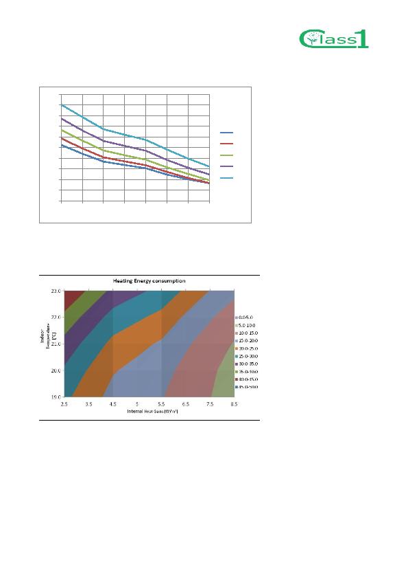
The simulation results can be shown also using a surface graph (see Figure 66) where each colour
represents a range o normalized space heating consumption, and where to each couple indoor
temperature-internal heat gain corresponds a normalized space heating consumption value.
Figure 66. Simulated space heating consumption by varying internal heat gains and indoor temperature: surface graph
representation.
Combining this surface graph representation to the LogLogistic probability distribution, it is possible to
calculate the probability related to each range of normalized space heating consumption (see Figure 67)
The heating consumption range with the highest probability is the 20-25 kWh/m
2
/y, with a probability of
29.2%. Each heating consumption range is related to a range of indoor temperature-internal gains couples.
This means, for instance, that there is a 29.2% probability that internal heat gains are the base value (5
W/m
2
) and that the indoor temperature varies between 20.5 and 21.7°C, or that the indoor temperature is
the base value (20°C) and that the internal heat gains vary between 3.6 and 4.6 W/m
2
.
0
5
10
15
20
25
30
35
40
45
50
2.5
3.5
4.5
5
5.5
6.5
7.5
8.5
H
e
ating
[kWh
/
m
2
]
Internal heat gain [W/m
2
]
19.0
20.0
21.0
22.0
23.0